
4 posts tagged with "wkt"

View All Tags

Visualising Indoor Spaces from OpenStreetMap in Power BI with Icon Map Pro

· 8 min read
Brynn Borton
Co-founder of Tekantis

When most people think of maps, they picture roads, rivers, and perhaps outlines of buildings. These are the features most visible in everyday map services, and they’re well covered in OpenStreetMap (OSM), a collaborative global project to create a free, editable map of the world. However, beyond the roads and rooftops, OSM contains a lesser-known layer of spatial data, indoor mapping.

In this article, we’ll explore how to unlock and visualise this hidden indoor data using Power Query and Icon Map Pro. We’ll focus on a couple of practical examples: a detailed hospital floor plan, and a shopping mall digital twin.

What is OpenStreetMap?

OpenStreetMap is often described as the “Wikipedia of maps.” Contributors around the world upload and refine geospatial data covering everything from buildings and highways to footpaths and forests. OSM data is open and freely available, making it a valuable foundation for many GIS and analytics applications.

What’s less known is that OSM also supports detailed indoor mapping through a structured tagging scheme. Tags such as indoor=room, level=, room=, and building:part allow contributors to define internal spaces such as hallways, offices, hospital rooms, and more. Some dedicated platforms, such as OpenLevelUp and indoor=, showcase this data, but it’s not typically exposed in standard maps.

Despite this, a surprising number of buildings have detailed internal mapping. Airports, train stations, universities, and hospitals are often rich with this hidden geometry, if you know where to look.

First Example: Hospital Floor Plans in Denver

We set out to see how much detail we could extract from OpenStreetMap for a real-world building. After exploring various cities, we discovered that a hospital in Denver, Colorado has been extensively mapped, with rooms, corridors, toilets, and walls all represented using the OSM indoor tagging model.

Using the Overpass API, we queried for all objects in a bounding box around the hospital that included tags like indoor=room, room=*, and level=*. This gave us a rich dataset of floor plans directly from the open map, structured as OSM way elements with sets of nodes forming closed loops.

The question then became: how do we transform this into something visual and interactive in Power BI?

Accessing OSM Data: Introducing Overpass and Overpass QL

Before diving into Power Query, it's important to understand how we extract data from OpenStreetMap. The Overpass API is a read-only API that allows users to query and extract subsets of OSM data using a powerful query language called Overpass QL. It supports filtering by tags, bounding boxes, and spatial relationships.

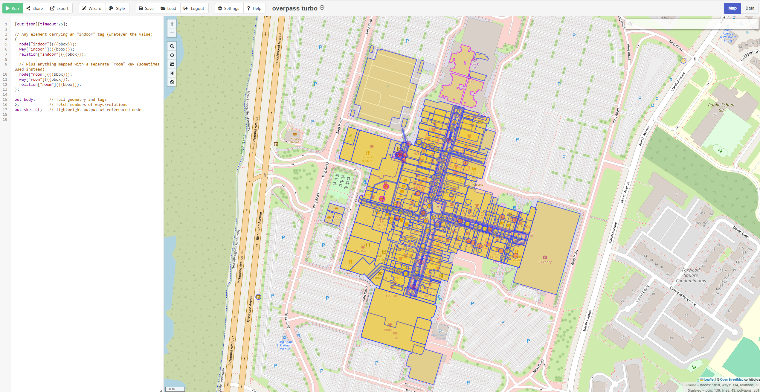
You can explore and test Overpass QL queries using the interactive editor at overpass-turbo.eu.

Here's a sample query that returns indoor-related elements:

[out:json][timeout:25];

// Any element carrying an "indoor" tag (whatever the value)
(
node["indoor"]({{bbox}});
way["indoor"]({{bbox}});
relation["indoor"]({{bbox}});

// Plus anything mapped with a separate "room" key (sometimes used instead)
node["room"]({{bbox}});
way["room"]({{bbox}});
relation["room"]({{bbox}});
);

out body geom; // full geometry and tags

Overpass Turbo

Extracting and Converting the Geometry in Power Query

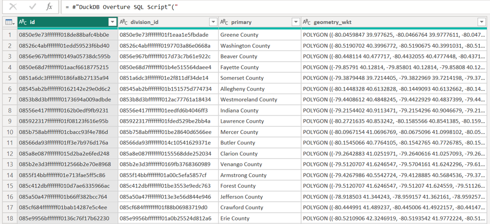
To load the data into Power BI, we created a Power Query function that sends the Overpass QL query to the API, receives the JSON response, and parses the elements into a table. We handle the processing of OSM geometry data by parsing it into WKT (Well-Known Text) format, which is natively supported by Icon Map Pro for rendering vector shapes in Power BI.

Here is an example Power Query snippet that call our function, there are also some additional cleaning steps we did:

let
Source = #"OSM Overpass Query"("[out:json][timeout:25];

// Any element carrying an ""indoor"" tag (whatever the value)
(
node[""indoor""](39.727719308804495,-104.99282167277055,39.729021993404594,-104.99005363306718);
way[""indoor""](39.727719308804495,-104.99282167277055,39.729021993404594,-104.99005363306718);
relation[""indoor""](39.727719308804495,-104.99282167277055,39.729021993404594,-104.99005363306718);

// Plus anything mapped with a separate ""room"" key (sometimes used instead)
node[""room""](39.727719308804495,-104.99282167277055,39.729021993404594,-104.99005363306718);
way[""room""](39.727719308804495,-104.99282167277055,39.729021993404594,-104.99005363306718);
relation[""room""](39.727719308804495,-104.99282167277055,39.729021993404594,-104.99005363306718);
);

out body; // full geometry and tags
>; // fetch members of ways/relations
out skel qt; // lightweight output of referenced nodes", null),
#"Extracted Values" = Table.TransformColumns(Source, {"nodes", each Text.Combine(List.Transform(_, Text.From), ","), type text}),
#"Filtered Rows" = Table.SelectRows(#"Extracted Values", each ([WKT] <> null) and ([type] = "way")),
#"Removed Columns" = Table.RemoveColumns(#"Filtered Rows",{"nodes", "members", "bounds", "lon", "lat"}),
#"Replaced Value" = Table.ReplaceValue(#"Removed Columns","toilet","toilets",Replacer.ReplaceText,{"tag_amenity"}),
#"Replaced Value1" = Table.ReplaceValue(#"Replaced Value","toiletss","toilets",Replacer.ReplaceText,{"tag_amenity"}),
#"Replaced Value2" = Table.ReplaceValue(#"Replaced Value1","bathroom","shower",Replacer.ReplaceText,{"tag_amenity"}),
#"Replaced Value3" = Table.ReplaceValue(#"Replaced Value2","toilet","toilets",Replacer.ReplaceText,{"tag_room"}),
#"Filtered Rows1" = Table.SelectRows(#"Replaced Value3", each ([tag_indoor] = "corridor" or [tag_indoor] = "room")),
#"Replaced Value4" = Table.ReplaceValue(#"Filtered Rows1","toiletss","toilets",Replacer.ReplaceText,{"tag_room"}),
#"Replaced Value5" = Table.ReplaceValue(#"Replaced Value4","bathroom","shower",Replacer.ReplaceText,{"tag_room"}),
#"Replaced Value6" = Table.ReplaceValue(#"Replaced Value5","meeting","examination",Replacer.ReplaceText,{"tag_room"}),
#"Replaced Value7" = Table.ReplaceValue(#"Replaced Value6","workshop","screening",Replacer.ReplaceText,{"tag_room"}),
#"Replaced Value8" = Table.ReplaceValue(#"Replaced Value7","lobby","reception",Replacer.ReplaceText,{"tag_room"}),
// If tag_room is null AND the corridor flag is present, set it to "corridor"
#"Set tag_room for corridors" =
let
Added = Table.AddColumn(
#"Replaced Value8",
"tag_room_tmp",
each if [tag_room] = null
and ( [type] = "corridor" or [tag_indoor] = "corridor" )
then "corridor"
else [tag_room],
type text
),
RemovedOld = Table.RemoveColumns(Added, {"tag_room"}),
Renamed = Table.RenameColumns(RemovedOld, {{"tag_room_tmp", "tag_room"}})
in
Renamed,
#"Removed Columns1" = Table.RemoveColumns(#"Set tag_room for corridors",{"tag_highway", "tag_note", "tag_local_ref", "tag_addr:city", "tag_addr:housenumber", "tag_addr:postcode", "tag_addr:state", "tag_addr:street", "tag_brand", "tag_brand:wikidata", "tag_cuisine", "tag_delivery", "tag_drive_through", "tag_opening_hours", "tag_outdoor_seating", "tag_phone", "tag_smoking", "tag_takeaway", "tag_website", "tag_website:menu", "tag_operator", "tag_shop", "tag_area", "tag_toilets:disposal", "tag_amenity", "tag_level"}),
#"Reordered Columns" = Table.ReorderColumns(#"Removed Columns1",{"type", "id", "geometry", "tag_access", "tag_room", "tag_indoor", "tag_name", "tag_ref", "tag_unisex", "tag_wheelchair", "tag_female", "tag_male", "WKT"})
in
#"Reordered Columns"

You may notice that the Overpass query uses {{bbox}}, while in Power Query we specify actual coordinates. {{bbox}} is a special placeholder in Overpass that represents the current visible area in tools like Overpass Turbo. To get the final query with real coordinates, simply click Export and choose Copy raw query.

Visualising the Result in Icon Map Pro

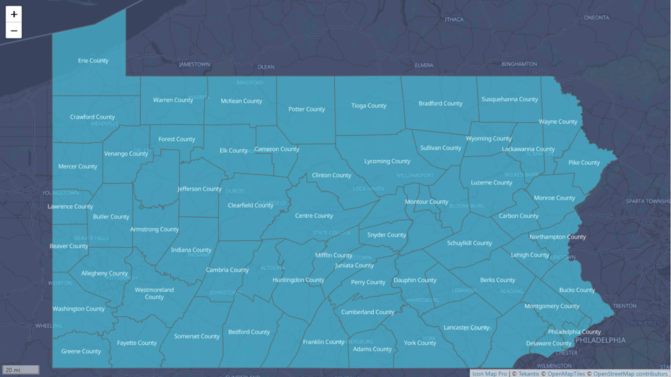
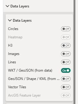
Once the WKT column is ready, it’s a simple matter of dropping it into Icon Map Pro, using the built in support for WKT layers.  The result? A full, zoomable, interactive floor plan of the hospital within Power BI.

Hospital Interactive Floor Plan

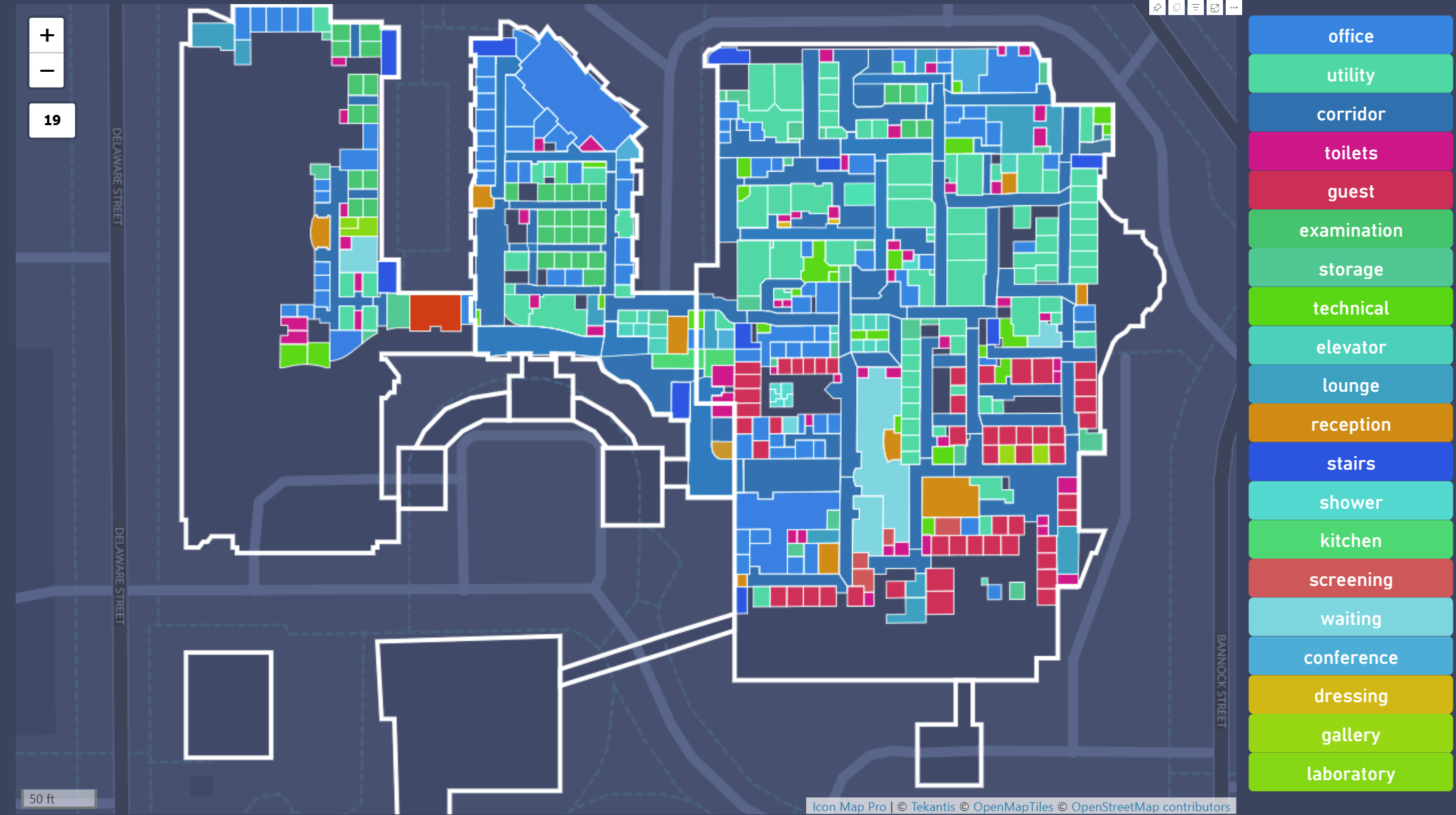
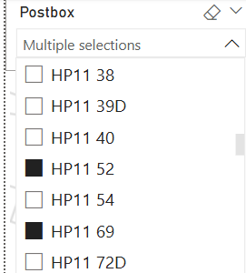
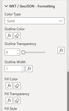
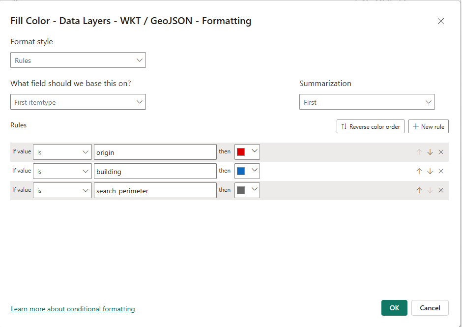
In this example, we are colouring rooms by type, adding basic tooltips with room metadata, and using the new Power Slicer visual as an interactive legend to dynamically filter the floor plan. While this is a simple demonstration, the same approach could be developed into a full digital twin solution for a hospital. For example, it could overlay sensor data such as room occupancy or air quality, integrate cleaning or maintenance schedules, highlight emergency routes, or track patient movements and staff locations in real time, the possibilities are endless. 

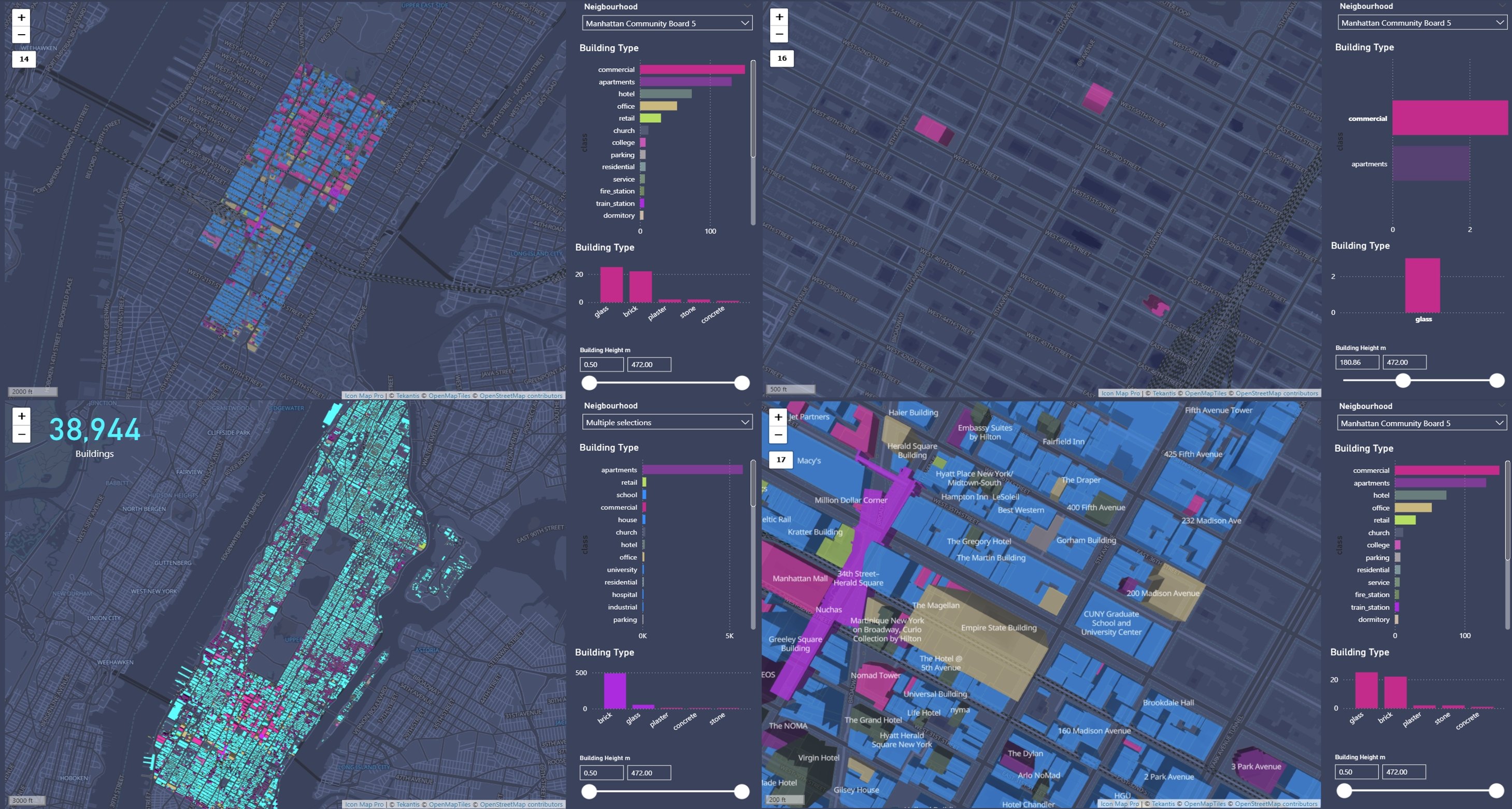
Example 2 – Shopping Mall

The hospital example worked well, but we also came across some highly detailed indoor maps of shopping malls. These were particularly interesting due to their multiple floors and extensive tagging. By repeating the same Overpass query pattern and incorporating a simple level slicer in Power BI, we were able to build a visual representation of a multi-storey shopping centre. In our demo, shops were displayed with vacant units clearly highlighted in pink.

Shopping Mall Digital Twin

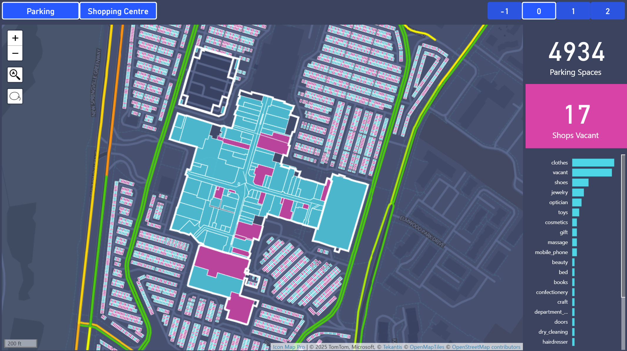
In addition to the floor plan, we discovered that the entire car park had been mapped in OSM, with each individual parking space represented as a polygon and tagged with parking=space. By running a second query and applying some AI-generated synthetic data (more on that in a future blog post), we visualised the car park occupancy, showing which spaces were in use and which were available.

To enhance the visual presentation, we downloaded a GeoJSON layer of the building outline, from OSM, and used it in Icon Map Pro as a Reference Layer, once as a simple white outline, and again as a filled roof polygon. We configured the roof layer to disappear beyond a certain zoom level, creating a subtle visual effect where the roof appears when zoomed out, but disappears to reveal the interior detail when zoomed in.     

To enhance the context further, we enabled Icon Map Pro’s live traffic layer to show real-time traffic delays around the shopping centre.

This approach could easily be developed into a comprehensive digital twin of the mall, combining spatial data with operational insights such as footfall heatmaps, tenant turnover, or even predictive maintenance for facilities.

Why This Matters

Icon Map Pro also supports images as backgrounds with x,y coordinates, which we have typically used for indoor mapping, see here for more details. Now, by incorporating structured OSM data and other geocoded sources like CAD exports, we can extend this capability into highly detailed micro-level location analysis. With the flexibility to zoom from room-level detail to a global view, users can create rich, scalable dashboards.

For example, a shopping mall operator could visualise all their malls around the world within one interactive Power BI report, drilling into each site for occupancy, tenant analytics, or maintenance schedules, all while retaining geographic context. The same principle applies across sectors, from healthcare estates to educational campuses and logistics hubs.

Conclusion

Indoor mapping in OpenStreetMap is a largely untapped resource, but it’s full of potential. By combining the flexibility of Power Query, the openness of Overpass API, and the rendering power of Icon Map Pro, we can bring this hidden data to life in Power BI.

Whether you're exploring hospitals, transport hubs, or university campuses, the indoor world is waiting to be mapped. While there is a growing amount of indoor data in OSM, it remains sparse compared to outdoor coverage. We hope this blog inspires more organisations to contribute detailed indoor data for their facilities, helping to build a richer, community-driven view of the world’s interior spaces.  

Overture Maps in Power BI using DuckDB & Icon Map Pro

· 15 min read
Brynn Borton
Co-founder of Tekantis

James Dales and I recently spoke at SQLBits about how geospatial analytics is transforming thanks to modern cloud-native formats. Our talk, "Geospatial Meets Big Data: Transforming Location Intelligence," provided insights into emerging technologies reshaping location analytics.

During our presentation, we demonstrated how DuckDB could be embedded within Power BI to unlock advanced geospatial capabilities. This blog expands on our SQLBits talk, offering a more detailed exploration and practical examples.

Introducing DuckDB: A Lightweight Powerhouse

DuckDB is an open-source, lightweight SQL database designed specifically for analytical workloads. Built for efficiency and ease of use, it runs directly within the host process with no need for a separate server, and can operate entirely in-memory or on disk as needed. Its columnar storage, vectorised execution, and minimal setup make it well-suited for modern, cloud-based analytics.

This lightweight and flexible architecture led us to explore DuckDB’s potential for enhancing geospatial data processing within Power Query, especially for scenarios where performance and portability are key.

Integrating DuckDB with Power Query

Our first step involved setting up the necessary drivers. We downloaded the DuckDB ODBC driver directly from their official site DuckDB ODBC Driver and installed it locally. While exploring connectivity options, we discovered MotherDuck's custom DuckDB connector for Power BI. Initially promising, we soon realised its limitations, it provided basic table access but lacked the ability to install the DuckDB geospatial libraries, executing custom SQL and required a physical instance of duck db on disk somewhere. Thus, we decided to handle connectivity manually using Power Query M scripts.

After a few minutes of tinkering, we achieved what we had hoped might be possible: spinning up a fully in-memory instance of DuckDB that lives entirely in RAM. This gives us all the power of DuckDB with zero files, zero server process, and zero install footprint. All that was needed was this simple one-line connection string:

ConnStr  = "Driver=DuckDB Driver;" &
"Database=:memory:;" &
"access_mode=read_write;" &
"custom_user_agent=PowerBI;",

Direct Access to Overture Data with DuckDB

Our initial practical use case was to dive straight into Overture Maps, a community-driven, open-source basemap project created collaboratively by Amazon, Microsoft, Meta, and TomTom, and hosted under the governance of the Linux Foundation. Overture provides comprehensive global map data, including detailed administrative boundaries, building footprints, transportation networks, points of interest, and more. This data is made available through regular monthly releases, which users can access directly from cloud storage platforms such as AWS S3 and Azure Blob. The diagram below provides an overview of Overture Maps' datasets and structure.

Overture Maps Overview Diagram

To make things easier, we developed a reusable Power Query function that sets up the DuckDB connection, installs the required libraries (spatial and httpfs), and provides a SQL placeholder ready for use. This allows seamless execution of DuckDB SQL and direct access to data from AWS S3.

(Note: While there is a version of Overture Maps hosted in Azure, we found the S3 version worked immediately, so we chose to use that.)

Here’s the Power Query function:

//////////////////////////////////////////////////////////////////////
// DuckDBQuery – execute arbitrary DuckDB SQL in an in-memory DB
// ---------------------------------------------------------------
// Parameters:
// sqlText (text, required) – your SELECT / DDL / DML script
// s3Region (text, optional) – defaults to "us-west-2"
//
//////////////////////////////////////////////////////////////////////
let
DuckDBQuery =
(sqlText as text, optional s3Region as text) as table =>
let
// ── 1. choose region (default us-west-2) ──────────────────────
region = if s3Region = null then "us-west-2" else s3Region,

// ── 2. one ODBC connection string to an in-memory DB ─────────
ConnStr = "Driver=DuckDB Driver;" &
"Database=:memory:;" &
"access_mode=read_write;" &
"custom_user_agent=PowerBI;",

// ── 3. build a single SQL batch: install, load, set, run ─────
BatchSQL =
Text.Combine(
{
"INSTALL spatial;",
"INSTALL httpfs;",
"LOAD spatial;",
"LOAD httpfs;",
"SET autoinstall_known_extensions=1;",
"SET autoload_known_extensions=1;",
"SET s3_region = '" & region & "';",
sqlText
},
"#(lf)" // line-feed separator
),

// ── 4. execute and return the result table ───────────────────
Result = Odbc.Query(ConnStr, BatchSQL)
in
Result
in
DuckDBQuery

Example: Extracting US County Boundaries

Using our custom function, we started by directly accessing the area boundaries from the Overture Divisions theme. Overture data is structured as a number of data themes. Each is stored as GeoParquet files in cloud storage, an enhanced version of the widely-used Apache Parquet format, which powers big data frameworks like Apache Spark and Trino. GeoParquet therfore blends geospatial processing capabilities with the high-performance analytics advantages of columnar data storage.

DuckDB is specifically optimised for this format and natively interacts with GeoParquet files directly in cloud environments using its built-in read_parquet function, thus enabling efficient spatial queries against massive datasets without additional data transformations or transfers.

For our first example, we extracted county boundaries within Pennsylvania, USA.  We also leveraged DuckDB's ST_AsText function to convert binary geometries (WKB) into readable WKT formats that are fully compatible with Power BI and Icon Map Pro.

let
Source = #"DuckDB Overture SQL Script"("
SELECT id,
division_id,
names.primary,
ST_AsText(geometry) AS geometry_wkt
FROM read_parquet(
's3://overturemaps-us-west-2/release/2025-01-22.0/theme=divisions/type=division_area/*',
hive_partitioning = 1
)
WHERE subtype = 'county'
AND country = 'US'
AND region = 'US-PA';", null)
in
Source

Here was the data returned:

Overture Divisions Data

The query executed in around 25 seconds, retrieving all 67 counties. This doesn't sound that impressive but when you consider the dataset contains over 5.5 million divisions within a 6.4GB GeoParquet file, accessed remotely from AWS cloud storage it's not bad at all.

Addressing Column Truncation Issues

Initially, our geometry data was truncated to 200 characters due to metadata handling limitations between Power Query and the DuckDB ODBC driver. When the ODBC driver does not expose column length information, Power BI defaults to a maximum of 200 characters for string columns. To resolve this, we explicitly cast our geometry data to a wider column type.

CAST(ST_AsText(geometry) AS VARCHAR(30000))

This ensured the most geometry polygons were retrieved successfully but a few were still over the 30000 character limit.

Simplifying the Polygons

To get all polygons under the limit we needed to simplify the polygons, luckily DuckDB has another handy function ST_SimplifyPreserveTopology.

Also to simplify usability, especially for analysts unfamiliar with SQL, we extended our PowerQuery function, allowing users to query Overture themes, specify column selections, conditions, and simplify polygons directly via function parameters.

//////////////////////////////////////////////////////////////////////
// OvertureQuery – default boundary simplification //
//////////////////////////////////////////////////////////////////////
let
OvertureQuery =
(
theme as text, //Overture maps theme
ctype as text, //Overture Maps Dataset
optional columnsTxt as nullable text, //list of columns, defaults to all
optional includeGeomWkt as nullable logical, //include the geometry as WKT
optional whereTxt as nullable text, //the where clause to filter the data
optional s3Region as nullable text, //options s3 region, defaults to us-west-2
optional simplifyTolDeg as nullable number // degrees tolerance, default 0.0005, 0=none
) as table =>
let
// ── defaults ────────────────────────────────────────────────
region = if s3Region = null then "us-west-2" else s3Region,
colsRaw = if columnsTxt = null or columnsTxt = "" then "*" else columnsTxt,
addWkt = if includeGeomWkt = null then true else includeGeomWkt,
tolDegDefault = 0.0005, // ≈ 55 m at the equator
tolDeg = if simplifyTolDeg = null then tolDegDefault else simplifyTolDeg,

// ── geometry expression ────────────────────────────────────
geomExpr = if tolDeg > 0
then "ST_SimplifyPreserveTopology(geometry, " &
Number.ToText(tolDeg, "0.############") & ")"
else "geometry",

// ── SELECT list ────────────────────────────────────────────
selectList = if addWkt
then Text.Combine(
{ colsRaw,
"CAST(ST_AsText(" & geomExpr & ") as VARCHAR(30000)) AS geometry_wkt" },
", ")
else colsRaw,

// ── WHERE clause (optional) ────────────────────────────────
whereClause = if whereTxt = null or Text.Trim(whereTxt) = ""
then ""
else "WHERE " & whereTxt,

// ── parquet URL ─────────────────────────────────────────────
parquetUrl =
"s3://overturemaps-" & region & "/" &
"release/2025-01-22.0/" &
"theme=" & theme & "/type=" & ctype & "/*",

// ── ODBC connection string (in-memory DuckDB) ──────────────
ConnStr =
"Driver=DuckDB Driver;" &
"Database=:memory:;" &
"access_mode=read_write;" &
"custom_user_agent=PowerBI;",

// ── SQL batch ───────────────────────────────────────────────
SqlBatch = Text.Combine(
{
"INSTALL spatial;",
"INSTALL httpfs;",
"LOAD spatial;",
"LOAD httpfs;",
"SET autoinstall_known_extensions = 1;",
"SET autoload_known_extensions = 1;",
"SET s3_region = '" & region & "';",
"",
"SELECT " & selectList,
"FROM read_parquet('" & parquetUrl & "', hive_partitioning = 1)",
whereClause & ";"
},
"#(lf)"
),

// ── run and return ──────────────────────────────────────────
OutTable = Odbc.Query(ConnStr, SqlBatch)
in
OutTable
in
OvertureQuery

Now we could easily invoke queries without writing any SQL and also simplify the polygons:

Source = #"DuckDB Overture Query with Simplify"(
"divisions",
"division_area",
"id, division_id, names.primary",
true,
"subtype = 'county' AND country = 'US' AND region = 'US-PA'",
null,
null)

We now have all polgons with a WKT string under the 30K limits, so we can easily visualise it in Icon Map Pro

Overture Divisions Data

Pushing the Limits: Querying 1.65 Million Buildings in NYC

Encouraged by initial success, we challenged DuckDB further using the significantly larger buildings dataset. Previously, querying these datasets using Apache Spark in Databricks resulted in poor performance. DuckDB, however, excelled even on our local laptop.

Now, we wanted to efficiently query buildings within a specific area, and the most effective way to do this is by using a bounding box. A bounding box defines a rectangular region with minimum and maximum coordinates, providing a quick way to filter geographic data. Ideally, we wanted to avoid manually calculating these coordinates. We noticed during our earlier exploration of the Overture divisions theme that each area already included a bbox column containing these coordinates. This gave us the idea to leverage these existing bounding boxes to easily geocode a city or area name. Once we had the bounding box, we could efficiently retrieve all buildings within that region by simply filtering based on these numeric values, eliminating the need for complex spatial queries.

The following is a Power Query function we created to easily retrieve a bounding box based on a city or area name and its standard 2-character ISO country code:

//////////////////////////////////////////////////////////////////////
// GetCityBBox – returns "lat1,lon1,lat2,lon2" for a settlement //
//////////////////////////////////////////////////////////////////////
let
GetCityBBox =
(
cityName as text, // e.g. "London"
isoCountry as text, // ISO-3166 alpha-2, e.g. "GB"
optional s3Region as nullable text
) as text =>
let
// ── query the locality polygon -----------------------------
rows =
OvertureQuery(
"divisions",
"division_area",
"bbox.xmin, bbox.ymin, bbox.xmax, bbox.ymax",
false, // no geometry_wkt
"subtype = 'locality' and " &
"country = '" & isoCountry & "' and " &
"names.primary ILIKE '" & cityName & "%'",
null, // no extra bounding box
s3Region, // defaults to us-west-2
0 // no simplification
),

// ── pick the first match (refine filter if ambiguous) -----
firstRow =
if Table.IsEmpty(rows)
then error "City not found in divisions data"
else Table.First(rows),

// ── assemble lat/lon string -------------------------------
bboxTxt =
Number.ToText(firstRow[bbox.ymin]) & "," &
Number.ToText(firstRow[bbox.xmin]) & "," &
Number.ToText(firstRow[bbox.ymax]) & "," &
Number.ToText(firstRow[bbox.xmax])
in
bboxTxt
in
GetCityBBox

Filtering with Bounding Boxes

We then modified our primary query function to include bounding box filtering capability:

//////////////////////////////////////////////////////////////////////
// OvertureQuery – with optional bounding box //
//////////////////////////////////////////////////////////////////////
let
OvertureQuery =
(
theme as text,
ctype as text,
optional columnsTxt as nullable text,
optional includeGeomWkt as nullable logical,
optional whereTxt as nullable text,
optional boundingBoxTxt as nullable text, // lat1,lon1,lat2,lon2
optional s3Region as nullable text,
optional simplifyTolDeg as nullable number // tolerance in degrees, 0 ⇒ none
) as table =>
let
// ── defaults ────────────────────────────────────────────────
region = if s3Region = null then "us-west-2" else s3Region,
colsRaw = if columnsTxt = null or columnsTxt = "" then "*" else columnsTxt,
addWkt = if includeGeomWkt = null then true else includeGeomWkt,
tolDegDefault = 0.0005, // ≈ 55 m at the equator
tolDeg = if simplifyTolDeg = null then tolDegDefault else simplifyTolDeg,

// ── geometry expression ────────────────────────────────────
geomExpr = if tolDeg > 0
then "ST_SimplifyPreserveTopology(geometry, " &
Number.ToText(tolDeg, "0.############") & ")"
else "geometry",

// ── SELECT list ────────────────────────────────────────────
selectList = if addWkt
then Text.Combine(
{ colsRaw,
"CAST(ST_AsText(" & geomExpr & ") AS VARCHAR(30000)) AS geometry_wkt" },
", ")
else colsRaw,

// ── optional bounding-box condition ───────────────────────
bboxCondRaw =
if boundingBoxTxt = null or Text.Trim(boundingBoxTxt) = "" then ""
else
let
nums = List.Transform(
Text.Split(boundingBoxTxt, ","),
each Number.From(Text.Trim(_))),
_check = if List.Count(nums) <> 4
then error "Bounding box must have four numeric values"
else null,
lat1 = nums{0},
lon1 = nums{1},
lat2 = nums{2},
lon2 = nums{3},
minLat = if lat1 < lat2 then lat1 else lat2,
maxLat = if lat1 > lat2 then lat1 else lat2,
minLon = if lon1 < lon2 then lon1 else lon2,
maxLon = if lon1 > lon2 then lon1 else lon2
in
"bbox.xmin >= " & Number.ToText(minLon, "0.######") &
" AND bbox.xmax <= " & Number.ToText(maxLon, "0.######") &
" AND bbox.ymin >= " & Number.ToText(minLat, "0.######") &
" AND bbox.ymax <= " & Number.ToText(maxLat, "0.######"),

// ── combine WHERE pieces ───────────────────────────────────
whereTxtTrim = if whereTxt = null then "" else Text.Trim(whereTxt),
wherePieces = List.Select({ whereTxtTrim, bboxCondRaw }, each _ <> ""),
whereClause = if List.Count(wherePieces) = 0
then ""
else "WHERE " & Text.Combine(wherePieces, " AND "),

// ── parquet URL ─────────────────────────────────────────────
parquetUrl =
"s3://overturemaps-" & region & "/" &
"release/2025-01-22.0/" &
"theme=" & theme & "/type=" & ctype & "/*",

// ── ODBC connection string (in-memory DuckDB) ──────────────
ConnStr =
"Driver=DuckDB Driver;" &
"Database=:memory:;" &
"access_mode=read_write;" &
"custom_user_agent=PowerBI;",

// ── SQL batch ───────────────────────────────────────────────
SqlBatch = Text.Combine(
{
"INSTALL spatial;",
"INSTALL httpfs;",
"LOAD spatial;",
"LOAD httpfs;",
"SET autoinstall_known_extensions = 1;",
"SET autoload_known_extensions = 1;",
"SET s3_region = '" & region & "';",
"",
"SELECT " & selectList,
"FROM read_parquet('" & parquetUrl & "', hive_partitioning = 1)",
whereClause & ";"
},
"#(lf)"
),

// ── run and return ──────────────────────────────────────────
OutTable = Odbc.Query(ConnStr, SqlBatch)
in
OutTable
in
OvertureQuery

Now we were ready to query the building outlines, along with a bunch of additional attributes that might be useful for further analysis. So let’s pull it all together and really put it to the test by attempting to extract all the buildings in New York City. We used our bounding box function to locate the spatial extent of the city, then passed this to our main query function.

let
NewYorkBBox = GetCityBBox("City Of New York", "US"),
NewYorkBuildings =
OvertureQuery(
"buildings",
"building",
"id, names.primary, class, height, subtype, class, num_floors, is_underground, facade_color, facade_material, roof_material, roof_shape, roof_color, roof_height",
true,
null,
NewYorkBBox,
null,
null
)
in
NewYorkBuildings

Amazingly, within around 5 minutes, we had extracted all 1.65 million buildings in New York City, complete with building outlines and a wealth of rich attributes. Even more impressive was that Power BI's resource usage remained minimal.

Spatial Joins: Assigning Buildings to Neighbourhoods

That is pretty cool, but even though Icon Map Pro can display up to half a million polygons on a map, 1.65 million buildings is just too many to visualise effectively. To manage this, we needed a way to filter buildings by area. Unfortunately, the Overture data does not provide a direct foreign key between buildings and divisions such as neighbourhoods, so we needed to perform a spatial join. No problem, however, because we can do exactly that using DuckDB's spatial functions.

This required switching back to SQL, as the query is more complex. We first selected the New York neighbourhoods from the division_area layer, then retrieved all the buildings within the city’s bounding box, and finally performed a spatial join using ST_Intersects to associate each building with its corresponding area.

let
Source = #"DuckDB Overture SQL Script"("
-- 1. Pull the New York City divisions you care about
WITH areas AS (
SELECT
id AS area_id,
names.primary AS area_name,
subtype,
geometry AS geom
FROM read_parquet(
's3://overturemaps-us-west-2/release/2025-01-22.0/theme=divisions/type=division_area/*',
hive_partitioning = 1
)
WHERE country = 'US'
AND region = 'US-NY'
AND subtype IN ('neighborhood')
),

-- 2. Load buildings inside the city’s overall bounding box first
bldg AS (
SELECT
id AS building_id,
names.primary AS building_name,
class,
height,
subtype,
class,
num_floors,
is_underground,
facade_color,
facade_material,
roof_material,
roof_shape,
roof_color,
roof_height,
geometry AS geom
FROM read_parquet(
's3://overturemaps-us-west-2/release/2025-01-22.0/theme=buildings/type=building/*',
hive_partitioning = 1
)
WHERE bbox.xmin > -74.3 AND bbox.xmax < -73.5
AND bbox.ymin > 40.4 AND bbox.ymax < 41.0
)

-- 3. Spatial join: which building sits in which area?
SELECT
a.area_name,
a.subtype,
b.building_id,
b.building_name,
b.class,
b.height,
b.subtype,
b.class,
b.num_floors,
b.is_underground,
b.facade_color,
b.facade_material,
b.roof_material,
b.roof_shape,
b.roof_color,
b.roof_height,
ST_AsText(b.geom) AS geometry_wkt
FROM bldg b
JOIN areas a
ON ST_Intersects(a.geom, b.geom);
", null),
#"Filtered Rows" = Table.SelectRows(Source, each true)
in
#"Filtered Rows"

Incredibly, we managed to join all 1.65 million rows in memory within Power BI on a standard laptop. Even more impressive, when monitoring system performance, Power BI Desktop was only using about 10% of CPU and under 4GB of memory, barely 1GB more than its normal baseline usage. Definitely some voodoo magic going on somewhere!

Visualising Results in Icon Map Pro

Finally, we visualised the results using Icon Map Pro within Power BI, colouring the buildings by type, and cross-filtering buildings by neighbourhood, type, height, and material properties.

Overture Maps Buildings Icon Map Pro

So, What's the Catch?

Currently, the only limitation is that DuckDB's ODBC driver isn't included by default in Power BI Service. Hence, similar to other third-party ODBC drivers, a Power BI Gateway server is required. Thankfully, setting this up is straightforward, simply spin up an Azure VM, install the DuckDB driver, and configure it as your gateway. You’ll then fully leverage DuckDB's capabilities in your Power BI cloud environment and be able to refresh on a schedule like any other data.

Explore the Possibilities

We encourage you to explore and innovate with this approach, leveraging Overture Maps or your own spatial datasets. Experiment freely and share your exciting findings with us!

You can download a copy of the PBIX file here which includes all the powerquery functions and some other goodies like using DuckDB for generating H3 hexagons, another blog post coming soon on that one!

Interactive Spatial Data Operations in Fabric SQL

· 8 min read
James Dales
Co-founder of Tekantis

With SQL Server now in public preview inside of Microsoft Fabric, I was keen to investigate it's spatial data functions. Whilst the Event House has provided spatial data processing inside of Fabric since the outset with KQL database, I was excited when the SQL engine arrived as it's a more familiar environment to those working with spatial data. It also opens up the door for doing realtime processing of that data based on interactions in a Power BI report.

Fabric SQL has strong support for geospatial datatypes and functions opening up a wide range of operations such nearest neighbours, distance calculations, boundary intersections etc etc.

In this example I wanted to keep things simple and show properties within a selected distance from selected postboxes. The postboxes would be selected by a Power BI slicer, as would the distance required. Then on making these selections, SQL server would then find the properties within those search radiuses.

alt text

First of all I needed some data to use, so I extracted from OpenStreetMap the locations of all the postboxes in Buckinghamshire in the UK using the QuickOSM plugin for QGIS. I also did the same for all the buildings in Buckinghamshire. There's only partial data for building outlines in Buckinghamshire, a better datasource for these would have probably been Ordnance Survey data. I saved these two separate data extracts in CSV format with WKT geometry.

So with my data ready, I headed over to Microsoft Fabric, and was quickly and easily able to create SQL database in just 2 clicks. Importing the data was also straightforward using DataFlows Gen 2 to upload the CSV file into OneDrive and import into 2 tables within the database using the familiar PowerQuery interface. The only downside here is that PowerQuery can't create fields of type geography so the WKT data is added as a text field. But this is quickly remedied once the data is loaded.

I also added spatial indexes on the columns containing the spatial data to improve performance.

alt text

With my data loaded I was now ready to create a function to to perform the spatial searches when triggered from Power BI. I opted to use a table function as I can then parameterize the search criteria using PowerQuery parameters - I've not been successful in achieving this with stored procedures.

From Power BI, I pass in a list of comma separated postbox references and the distance in meters to search. The first thing we need to do is process that list of postboxes:

WITH RefList AS (
SELECT TRIM(value) AS ref FROM STRING_SPLIT(@Ref, ',')
)

With that done we can use the STDistance spatial function to calculate the distance between the buildings and the selected postboxes, and return those within the specified distance:

-- Return buildings where the distance from the postboxes is less than @Distance
SELECT
b.full_id,
b.geom.STAsText() AS WKT,
b.building,
'building' AS itemtype
FROM dbo.buildings AS b INNER JOIN dbo.postboxes AS p ON p.ref IN (select ref from RefList)
WHERE b.geom.STDistance(p.geom) <= @Distance

As well as showing the matched properties in the results, I also wanted to show the locations of the postboxes, so we use a UNION ALL to add the postbox locations into the results:


UNION ALL

-- Return a points for the postbox locations
SELECT
full_id,
p2.geom.STAsText() AS WKT,
'' AS building,
'origin' AS itemtype
FROM dbo.postboxes AS p2
WHERE p2.ref IN (select ref from RefList)

And then finally I also wanted to return the search radius to show on the map:

UNION ALL

-- Return the perimeter of the search areas as polygons
SELECT
p3.ref + 'perimeter' AS full_id,
p3.geom.STBuffer(@Distance).STAsText() AS WKT,
'' AS building,
'search_perimeter' AS itemtype
FROM dbo.postboxes AS p3
WHERE p3.ref IN (select ref from RefList)

Here's the complete function:


ALTER FUNCTION dbo.fn_GetBuildingsWithinDistance
(
@Ref nvarchar (4000),
@Distance FLOAT
)
RETURNS TABLE
AS
RETURN
(

WITH RefList AS (
SELECT TRIM(value) AS ref FROM STRING_SPLIT(@Ref, ',')
)

-- Return buildings where the distance from the postboxes is less than @Distance
SELECT
b.full_id,
b.geom.STAsText() AS WKT,
b.building,
'building' AS itemtype
FROM dbo.buildings AS b INNER JOIN dbo.postboxes AS p ON p.ref IN (select ref from RefList)
WHERE b.geom.STDistance(p.geom) <= @Distance

UNION ALL

-- Return a points for the postbox locations
SELECT
full_id,
p2.geom.STAsText() AS WKT,
'' AS building,
'origin' AS itemtype
FROM dbo.postboxes AS p2
WHERE p2.ref IN (select ref from RefList)

UNION ALL

-- Return the perimeter of the search areas as polygons
SELECT
p3.ref + 'perimeter' AS full_id,
p3.geom.STBuffer(@Distance).STAsText() AS WKT,
'' AS building,
'search_perimeter' AS itemtype
FROM dbo.postboxes AS p3
WHERE p3.ref IN (select ref from RefList)
);

This is all the setup required within Fabric SQL, so now over to Power BI Desktop.

I was able to connect to Fabric SQL in the same way as I'd connect to any SQL DB, so that was easy, and I simply imported the postbox table as import mode into my Power BI model. I was't worried about any geometry here, just the reference numbers, although in real life, I'd have imported additional reference data for improved searching and selection.

Now to bring in the building search results. I next made to parameters in PowerQuery used to pass the selected postboxes and the search distance.

alt text

Now we're ready to create the connection to the table function. As we want the searching to be done interactively, we need to ensure the connection to the table function is made using Direct Query. This means that the SQL query is executed and new results returned every time we interact with the slicers (or other visuals) in the report.

After making the initial connection, I then edited the query in the Advanced Editor. This is because we need to add a little code to handle the multi-selection of postboxes. There's likely a better approach for this, but this seems to work well. First of all I handle a single value vs multiple, and then create a comma separated text string with the selected values:

alt text

Note we're using the parameters postbox_ref and range that I configured earlier.

Here's the M code:

let
// Normalize postbox_ref to a list if it's a single string
normalizedList = if Value.Is(postbox_ref, type list) then postbox_ref else {postbox_ref},

// Combine into a single comma-separated string
commaSeparated = Text.Combine(normalizedList, ","),

Source = Sql.Database("yourdatabaseservergoeshere.database.fabric.microsoft.com", "spatialsql-314d84ad-21da-438c-9caf-76f51b7259d9"),
dbo_fn_GetBuildingsWithinDistance = Source{[Schema="dbo",Item="fn_GetBuildingsWithinDistance"]}[Data],
#"Invoked Functiondbo_fn_GetBuildingsWithinDistance1" = dbo_fn_GetBuildingsWithinDistance(commaSeparated, range)
in
#"Invoked Functiondbo_fn_GetBuildingsWithinDistance1"

That's the data connections sorted. Now over to Power BI's report editor. The queries should load in all the postbox references into a table, and the table function should be called using the default values defined in the PowerQuery parameters.

We now need to set up the interactivity part of the report. So I added a slicer based on the post code reference.

alt text

But this won't currently change how the table function is called - we need to link up this to the Power Query function. We do this in the Power BI Model View.

Selecting the postcode reference field on the right, shows the properties panel. We need expand the Advanced section and in the "Bind to parameter" section, select our PowerQuery postbox_ref parameter. And then also enable Multi-Select.

alt text

This then binds this field to the PowerQuery parameter. When we select an item in the slicer now, that value is passed into the SQL query.

We also need to do something similar for the distance selection. For this I created a numeric range parameter:

alt text

alt text

This then provides us with a table of numbers, and a slicer, but we need to bind it to the PowerQuery parameter before we can use it. So back in the Model view, bind it to the range parameter a we did for the postbox_ref parameter, but this time don't enable Multi-select:

alt text

And now we're ready to display the results, which of course I used Icon Map Pro for.

The field configuration is straight forward, I add the full_id field into the ID field, and the geom field into the Image / WKT field:

alt text

Then in formatting settings for Icon Map Pro, in the Data Layers I just enabled WKT / GeoJson (from data):

alt text

And set up some conditional formatting for the buildings vs the postboxes and search radius:

alt text

eg:

alt text

Here's a video showing it in action:

Bus Routes

· 2 min read
James Dales
Co-founder of Tekantis

During the recent 30 Day Map Challenge I published a report with many of Europe's railway routes, which gained a lot of interest. I thought I'd see whether the same thing was possible for bus routes.

I'd sourced the data for the railway networks from OpenStreetMap, but it seems OpenStreetMap doesn't have sufficient data for bus routes - it's either inconsistent or partially populated.

However, I found that the Department for Transport has a Bus Open Data Site. This seems a great source of data, and I've only had chance to scratch the surface. I've started with timetable data. There's a lot of it! For starters, buses stop a lot more than trains, so there are a lot more stops, and the coordinates between each stop along the routes are detailed, as again, roads have many more turns (and roundabouts!) than railway lines.

The data downloads are large, so I've focussed on just one operator for now, the GoAhead group and downloaded their timetable data for the North East. This report represents all of their routes. A Power BI slicer enables you to pick a route, or alternatively you can search for a specific stop and all the routes that service that stop will be displayed. The chosen stop is highlighted in red.

alt text

Hovering over a stop with the mouse cursor will display the timetable information for all the buses that service that stop.

alt text

There are complexities, and nuances in the data that I haven't represented in the report, but it was a good proof of concept to see what could be achieved with bus data in a few hours. I see there's an API to retrieve the realtime locations of buses, so I'm looking forward to an excuse to explore that!